
In Search of g
While most variables used in motivating the asset valuation models in this study are either derived from primary input data or forecast using expected changes in firm operations and market conditions, one variable with particular impact on most model outcomes is g, the expected growth rate of the model’s subject cash flow variable applied in the continuing value portion of the model. As this part of the equation is an algebraic derivation of an infinite series of cash flows, growing at a given rate in perpetuity, the assignment of an aggressive value for g results in unreasonable model outcomes. For example, were we to assume a long-run growth rate of 20%, a feat not observed in modern finance for more than a few years at a time for any publicly traded firm, the model outcome would be so large as to be completely unrealistic. However, if we assume a growth rate that does not take into account the potential for the firm’s management to innovate, invest, and provide ongoing improvement to the firm’s operating efficiency, we significantly understate the firm’s potential value to its stakeholders and the market generally.
This study includes valuation outcomes resulting from the use of three distinct versions of potential growth of the firm’s cash flow variables: g = % Δ GDP, g = IR x ROIC, and the g inferred when the valuation uses Enterprise Value (EV) as the firm’s value and then solves for g, referred to as the g solution throughout this study.
g = % Δ GDP
A reasonable expectation for a firm’s long-run cash flow might be its expansion at the rate of change of GDP (% Δ GDP), embodying some level of expected inflation and real economic growth. While this might not be terribly satisfying to investors in the long-run, it avoids the problem arising from the use of an overly optimistic value for g and the resulting unrealistic valuation estimate. Using a relatively nominal value for g in the continuing value portion of the valuation equation also reduces the potential for the model to result in a spurious valuation due to a negative denominator value when g is greater than WACC. This study uses g = % Δ GDP = 2.50% where seeking to motivate valuation models with a modest and exogenous level of g.
g = IR x ROIC
One of the textbook descriptions of the growth rate of a firm’s cash flow variable is that g is equal to the firm’s Investment Rate (IR) multiplied by its Return on Invested Capital (ROIC), or g = IR x ROIC. This forms an endogenous version of g resulting from the internal condition of the firm and its management’s decisions. While this form of g often results in relatively high values compared to g = % Δ GDP and is more likely to result in a spurious valuation estimate when g < WACC, but it is an observable level of g that might reasonably be thought of as a potential rate of growth to which the firm and its management might aspire.
g Solution
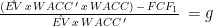
A firm’s Enterprise Value (EV) is expressly assigned by economic agents in the markets as equity shares and bonds are traded in a bid/ask process on open market exchanges, and it is this same EV we seek to estimate when employing an asset valuation model – it is the value of the firm’s stakeholder investments expressed as the present value of its future cash flows. If we substitute EV for the model outcome or estimate and then rearrange the model equation to solve for g, this allows us to observe the growth rate of the firm’s subject cash flow variable as inferred by the market’s establishment of the firm’s value. Which happens to be a very interesting observation.
We’ll use the Free Cash Flow Model (FCF) as an example. We know that EV is an observed value for the subject firms in this study as of a particular date; 

ROIC, WACC and NOPLAT are simply derived values based on the identities 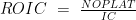


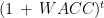
With 


The remaining equation is the continuing value equation, in this case expressed as 

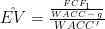
When this synthesized g is substituted into the valuation equation, the model outcome is equal to the firm’s enterprise value, as established by the market.