Models

Key Value Driver Model (KVD)	Free Cash Flow Model (FCF)	Economic Profit Model (Eπ)
Adjusted Present Value Model (APV)	Forward Market Multiple (FMM)

Key Value Driver Model (KVD)¹

Model Form

${ Value }_{ NOPLAT/KVD }=\sum { \frac { NOPLAT_{ t } }{ { \left( 1+WACC \right) }^{ t } } +\frac { \frac { { NOPLAT }_{ 1 }\left( 1-\frac { g }{ ROIC } \right) }{ WACC-g } }{ { \left( 1+WACC \right) }^{ t } } }$

${ Value }_{ FCF/KVD }=\sum { \frac { FCF_{ t } }{ { \left( 1+WACC \right) }^{ t } } +\frac { \frac { { NOPLAT }_{ 1 }\left( 1-\frac { g }{ ROIC } \right) }{ WACC-g } }{ { \left( 1+WACC \right) }^{ t } } }$

Inputs

Free Cash Flow (FCF)	$FCF\,=NOPLAT\,+\,Non-Cash\,\,Expenses-\Delta NWC\,-\,NCS$
Net Operating Profit Less Adjusted Taxes (NOPLAT)	$NOPLAT\,\,=\,\,EBIT\,\,*\,\,(\,\,-\,\,T)$
Invested Capital (IC)	$IC\,\,=\,\,Fixed\,\,Assets\,\,+\,\,Net\,\,Working\,\,Capital$
Return on Invested Capital (ROIC)	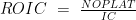$ROIC\,\,=\,\,\frac{NOPLAT}{IC}$
Weighted Average Cost of Capital – Market Based (WACC)	$WACC\,=\,\frac { E }{ V } { R }_{ E }\,+\,\frac { P }{ V } { R }_{ P }\,+\,\frac { D }{ V } { R }_{ D }\left( 1- Avg\,\, Tax\,\,Rate\,\,on\,\,Pre-Tax\,\,Income \right)$
Long-Run Growth Rate of Cash Flow Variable (g)	Long-run growth rates of the income variable (g = IR x ROIC and g = % $\Delta$ GDP) are used in the Continuing Value portion of the valuation models.

Description

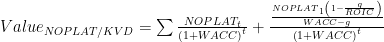
The Key Value Driver (KVD) model employed in this study includes an explicit forecast period during which relevant cash-flow variables are forecast and discounted to a present value, and a continuation period in which the firm’s terminal value is estimated through the use of key value drivers of the firm’s long run value creation. These key value drivers include NOPLAT, FCF, ROIC, WACC, and an estimation of the firm’s expected long-run growth rate (g).

While most iterations of this model form employ FCF during the explicit forecast period, some model examples suggest NOPLAT is preferable – in this study both are used and displayed.

The KVD model’s continuation term relies on a particular form of a free cash flow equation in which $FCF\,\,=\,\,NOPLAT\,\,x\,\,(1-\frac{g}{ROIC})$ .

This term forms the numerator in the continuing value equation $VAL_{CV(KVD)}\,\,=\,\,\frac{FCF}{WACC\,\, -\,\, g}\,\,=\,\,\frac{NOPLAT_{1}\,x\,(1\,\,-\,\frac{g}{ROIC})}{WACC\,\,-\,\,g}$

This model form brings the relationship between a firm’s of Return on Invested Capital (ROIC) and Weighted Average Cost of Capital (WACC) into focus. When the condition ROIC > WACC > g is present, the model provides consistently positive results. However, when WACC < g or ROIC < g, the model may provide spurious results and yield a negative outcome.

¹Richard Haskell, PhD (2017), Associate Professor of Finance, Bill & Vieve Gore School of Business, Westminster College, Salt Lake City, Utah, rhaskell@westminstercollege.edu, www.richardhaskell.net. Bryce Nieberger (2017), Student, Bill and Vieve Gore School of Business, Westminster College, Salt Lake City, Utah, http://www.linkedin.com/in/bryce-nieberger-91571ab7

Return to top of page

Free Cash Flow Model (FCF)¹

Model Form

VAL_FCF $= \sum { \frac { FCF_{ i } }{ { \left( 1+{ WACC} \right) }^{ t } } +\frac { \frac { { FCF }_{1 }}{ { WACC}-g } }{ { \left( 1+{ WACC} \right) }^{ t } } }$

Inputs

Free Cash Flow (FCF)	$FCF\,=NOPLAT\,+\,Non-Cash\,\,Expenses-\Delta NWC\,-\,NCS$
Long-Run Growth Rate of Cash Flow Variable (g)	Long-run growth rates of the income variable (g = IR x ROIC and g = % $\Delta$ GDP) are used in the Continuing Value portion of the valuation models.
Weighted Average Cost of Capital (Market Based)	$WACC\,=\,\frac { E }{ V } { R }_{ E }\,+\,\frac { P }{ V } { R }_{ P }\,+\,\frac { D }{ V } { R }_{ D }\left( 1- Avg\,\, Tax\,\,Rate\,\,on\,\,Pre-Tax\,\,Income \right)$

Description

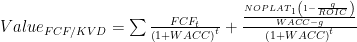
Among discounted cash flow models, those using Free Cash Flow (FCF) as the cash flow variable are most commonly used by analysts and practitioners. FCF is considered by some to be a more reliable performance measure than other income variables. It is also more reflective of the cash flow form for which the owners of the firm’s capital structure hold future rights. Further, FCF may be dis-aggregated such that it’s possible to focus specifically on the operational structure of the firm.

The advantage to this approach is obvious in that it allows for the calculation of a firm’s value based on that which the firm produces for its debt and equity stakeholders: free cash flow. The FCF valuation model considers the firm’s weighted average cost of capital (WACC) as the discounting factor and like other discounted cash flow models in this study is comprised of the sum of the present value of the discounted cash flows over an explicit forecast period and the present value of the firm’s continuing value using a Free Cash Flow augmented form of the Dividend Yield model.

Though technically robust, the continuing value portion of this model form includes a structural weakness observable when the firm’s WACC is less than its g, resulting in a negative denominator and almost certainly a negative outcome for the continuing value term; unless the cash flow variable in the numerator is also negative. This condition results in a spurious valuation, regardless of the length of the explicit forecast period.

¹ Prepared by Richard Haskell, PhD [2017], (Associate Professor of Finance, Bill & Vieve Gore School of Business, Westminster College, Salt Lake City, Utah, rhaskell@westminstercollege.edu, www.richardhaskell.net) and Beau Lewis [2017], (Undergraduate Research Associate, Finance, Bill and Vieve Gore School of Business, Westminster College, Salt Lake City, Utah, http://www.linkedin.com/in/beau-lewis-5068a5120)

Return to top of page

Economic Profit Model (Eπ)¹

Model Form

${ Value }_{ { ECON\pi } }={IC }_{ 0 }\,+\,\sum { \frac { { IC }_{ t }(ROI{ C }-WACC) }{ { \left( 1+WACC \right) }^{ t } } +\frac {\frac { {IC}_{0}\, (ROIC\,-\, WACC) }{ WACC-g } }{ { \left( 1+WACC \right) }^{ t } } }$

Inputs

Net Operating Profit Less Adjusted Taxes (NOPLAT)	$NOPLAT\,\,=\,\,EBIT\,\,*\,\,(1\,-\,T)$
Invested Capital (IC)	$IC\,\,=\,\,Fixed\,\,Assets\,\,+\,\,Net\,\,Working\,\,Capital$
Return on Invested Capital (ROIC)	$ROIC\,\,=\,\,\frac{NOPLAT}{IC}$
Weighted Average Cost of Capital – Market Based (WACC)	$WACC\,=\,\frac { E }{ V } { R }_{ E }\,+\,\frac { P }{ V } { R }_{ P }\,+\,\frac { D }{ V } { R }_{ D }\left( 1- Avg\,\, Tax\,\,Rate\,\,on\,\,Pre-Tax\,\,Income \right)$
Long-Run Growth Rate of Cash Flow Variable (g)	Long-run growth rates of the income variable (g = IR x ROIC and g = % $\Delta$ GDP) are used in the Continuing Value portion of the valuation models.

Description

The Economic Profit Model is a form of a discounted cash flow model that does not use an express cash flow, rather, it uses a synthesized cash flow represented by the spread between a firm’s Return on Invested Capital (ROIC) and its Weighted Average Cost of Capital (WACC). It also differs in that the explicit forecast period value is the sum of the firm’s Invested Capital (IC) at t = 0 and the discounted present value of the synthesized economic profit for the forecast years.

This model is as sensitive to time signatures as any in the study and suffers from the problematic relationship between WACC and g in the continuation term’s denominator. However, it is favored by many analysts and has a private market counterpart referred to as an Economic Value Added Model (EVA).

More clearly than any other model in the study, the Economic Profit model illustrates the effect of a firm’s value as a function of its ROIC and WACC. When ROIC > WACC growth adds value to the firm, when ROIC < WACC, growth destroys value.

Return to top of page

Adjusted Present Value Model (APV)¹

Model Form

VAL_APV $= \sum { \frac { FCF_{ i } }{ { \left( 1+{ k }_{ u } \right) }^{ t } } +\frac { \frac { { FCF }_{1 }}{ { k }_{ u }-g } }{ { \left( 1+{ k }_{ u } \right) }^{ t } } } +\sum { \frac { { TS }_{i } }{ { \left( 1+{ k }_{ tax } \right) }^{ t } } +\frac { \frac { { TS }_{1}}{ { k }_{ tax }-g } }{ { \left( 1+{ k }_{ tax } \right) }^{ t } } }$

Inputs

Free Cash Flow (FCF)	$FCF\,=\,NOPLAT\,+\,Non-Cash\,\,Expenses\,-\Delta\, NWC\,-\,NCS$
Tax Shield (TS)	$TS\,=\,Interest\,\,Paid\,\,x\,\,Avg\,\,Tax\,\,Rate\,\,on\,\,Pre-Tax\,\,Income$
Long-Run Growth Rate of Cash Flow Variable (g)	Long-run growth rates of the income variable (g = IR x ROIC and g = % $\Delta$ GDP) are used in the Continuing Value portion of the valuation models.
Unlevered Cost of Equity Capital (k_u)	This study employs the simplifying assumption that k_u= k_d= k_tax= WACC
Weighted Average Cost of Capital (Market Based)	$WACC\,=\,\frac { E }{ V } { R }_{ E }\,+\,\frac { P }{ V } { R }_{ P }\,+\,\frac { D }{ V } { R }_{ D }\left( 1- Avg\,\, Tax\,\,Rate\,\,on\,\,Pre-Tax\,\,Income \right)$

Description

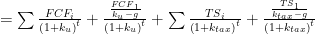
The Adjusted Present Value (APV) model takes into account the net present value of a firm asset inclusive of the valuation effects resulting from the firm’s choice of capital structures. It combines a Free Cash Flow valuation using the unlevered cost of equity (k_U) as its discount rate and a valuation using the firm’s tax shield (TS) arising from the interest costs associated with the firm’s debt capital using the firm’s opportunity cost of funds used to pay taxes as the discount rate (k_tax).

A primary purpose of this model form is to highlight changes in value as a function of changes in the firm’s capital structure, allowing for modeling with varying combinations of debt and equity capital. Though not expressly unique in this purpose, the APV model is the only one of the major discounted cash flow models to offer this perspective and is often used by practitioners seeking to present the case that the manner in which a firm is capitalized directly impacts the firm’s value.²

The APV model separates the value of forecasted free cash flows from the forecasted tax shields based on the premise that a tax shield (reduction of tax liability as the result of a tax deductible interest expense) has a similar effect on firm value as some other cash flow. The two segments of the equation, referred to commonly as V_FCF and V_TAX are presented as follows:

VAL_APV = VAL_FCF + VAL_TAX

VAL_FCF 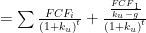$= \sum { \frac { FCF_{ i } }{ { \left( 1+{ k }_{ u } \right) }^{ t } } +\frac { \frac { { FCF }_{1}}{ { k }_{ u }-g } }{ { \left( 1+{ k }_{ u } \right) }^{ t } } }$ VAL_TAX $= \sum { \frac { { TS }_{ i } }{ { \left( 1+{ k }_{ tax } \right) }^{ t } } +\frac { \frac { { TS }_{1 }}{ { k }_{ tax }-g } }{ { \left( 1+{ k }_{ tax } \right) }^{ t } } }$

VAL_APV $= \sum { \frac { FCF_{i } }{ { \left( 1+{ k }_{ u } \right) }^{ t } } +\frac { \frac { { FCF }_{1 }}{ { k }_{ u }-g } }{ { \left( 1+{ k }_{ u } \right) }^{ t } } } +\sum { \frac { { TS }_{ i } }{ { \left( 1+{ k }_{ tax } \right) }^{ t } } +\frac { \frac { { TS }_{1 }}{ { k }_{ tax }-g } }{ { \left( 1+{ k }_{ tax } \right) }^{ t } } }$

The model uses a classic summative present value of the discounted cash flows added to the present value of the continuing value of the same cash flow form based on a cash flow augmented form of the Dividend Yield Model. This model form is employed using both the subject firm’s Free Cash Flow and Tax Shield, summed to form an Adjusted Present Value valuation.

Though technically robust, the continuing value portion of this model form includes a structural weakness observable when the firm’s WACC is less than g, resulting in a negative denominator and almost certainly a negative outcome for the continuing value term; unless the cash flow variable in the numerator is also negative. This condition results in a spurious valuation, regardless of the length of the explicit forecast period.

In this construction, an assumption of k_u = k_d (the levered cost of firm debt capital) is aligned with the firm having a constant debt to equity ratio, while an assumption of k_u = k_tax suggests a non-constant debt to equity ratio³. It’s important to note that the g in the continuing value equations represent the growth rate of the relevant cash flow variable.

² This is in direct contrast with the Modigliani and Miller Theorem in which the firm’s capital structure is said to have no impact on the firm’s value. This section of the theorem includes the assumption that interest and corporate income tax rates are held constant at 0%.

³ These assumptions arise from the Modigliani and Miller Theorem; Koller, T. Goedhart, M.H, Wessels, D., & Copeland, T.E.(2010), Valuation: Measuring and managing the value of companies (5^th Edition), pg. 122, Hoboken, NJ, John Wiley & Sons

Return to top of page

Forward Market Multiple Model (FMM)¹

Model Form

${ Value }_{ DCF/FMM}=\sum { \frac { FCF_{ t } }{ { \left( 1+WACC \right) }^{ t } } +\frac { { EBIT }_{ 1 }\,{x}\,{FMM}}{ { \left( 1+WACC \right) }^{ t } } }$ ${; \,\,FMM\,=\,\frac{{EV}_{t=0}}{{EBIT}_{t=0}}}$

Inputs

Free Cash Flow (FCF)	$FCF\,=NOPLAT\,+\,Non-Cash\,\,Expenses-\Delta NWC\,-\,NCS$
Earnings Before Interest and Taxes (EBIT)	$EBIT \,=\,Earnings\,\,Before\,\,Interest\,\,\&\,\,Taxes$
Net Operating Profit Less Adjusted Taxes (NOPLAT)	$NOPLAT\,\,=\,\,EBIT\,\,*\,\,(1\,-\,T)$
Invested Capital (IC)	$IC\,\,=\,\,Fixed\,\,Assets\,\,+\,\,Net\,\,Working\,\,Capital$
Return on Invested Capital (ROIC)	$ROIC\,\,=\,\,\frac{NOPLAT}{IC}$
Weighted Average Cost of Capital – Market Based (WACC)	$WACC\,=\,\frac { E }{ V } { R }_{ E }\,+\,\frac { P }{ V } { R }_{ P }\,+\,\frac { D }{ V } { R }_{ D }\left( 1- Avg\,\, Tax\,\,Rate\,\,on\,\,Pre-Tax\,\,Income \right)$
Long-Run Growth Rate of Cash Flow Variable (g)	Long-run growth rates of the income variable (g = IR x ROIC and g = % $\Delta$ GDP) are used in the Continuing Value portion of the valuation models.

Description

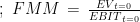
A valuation multiple is simply a ratio through which we view the value of the firm as a function of one if its inputs. These ratios, most often a quotient including some notion of the firm’s value interacted with an income based variable, offer a comparative metric useful for many reasons, not the least being a sense of the firm’s relative position among a group of peers. While on the surface this may appear to be more about a comparative metric, what underlies the ratio, or multiple, is a complex series of calculations and outcomes informing knowledgeable investors and analysts of the firm’s value.

Valuation multiples are often used to determine the value of an asset and as a single-stage multiple may also be thought of as a simplified valuation model. If we know the values for Enterprise Value (EV) and Earnings Before Interest and Taxes (EBIT) we can identify a multiple value as 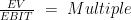$\frac{EV}{EBIT}\,\,=\,\,Multiple$ .

However, if we know EBIT and have a target for what the multiple value should be, we can synthesize an expected EV at a given point in time by multiplying the expected EBIT for that same point in time by an observed or target multiple. In this case we use a single-stage multiple in a single stage valuation model and no discounting for time or rate are required.

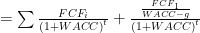
We can extend the use of a multiple to a continuation value applied after the end of an explicit forecast period in a dual-stage valuation model,

${ Value }_{ DCF/FMM}=\sum { \frac { FCF_{ t } }{ { \left( 1+WACC \right) }^{ t } } +\frac { { EBIT }_{ 1 }\,{x}\,\frac{{EV}_{t=0}}{{EBIT}_{t=0}}}{ { \left( 1+WACC \right) }^{ t } } }$ .

While there are numerous valuation multiple forms, in this study we consider a Forward Market Multiple Model employing FCF as the cash flow variable in the explicit forecast period and EV/EBIT as the multiple in the continuation period – a single-stage multiple used in a multi-stage valuation model.

A strength of using a market multiple as the continuing value is its simplicity and its avoidance of the problem we observe in some other continuing value forms in which the denominator includes the term WACC – g. When g > WACC we have an expressly negative term and possibly a spurious result. When using a multiple, the only way to obtain a negative result is for the cash flow variable to be negative, in which case the result is credible.

Return to top of page