
Models & Metrics
.
| Models and Metrics | Discounted Cash Flow (DCF) Models | Time Signatures |
Models and Metrics1
The models and metrics employed in the Valuation Project are those commonly used in corporate finance and investment banking. This study recognizes the three commonly constructed means of considering the value of an asset or firm, including its book value, market value, and production value. While accountants are most likely to be those interested in an asset’s book value (purchase cost less accumulated depreciation), bankers and economists tend to focus on market values. Interestingly enough, both book and market values are functions of an asset’s production value as it is this value that informs market values and sets initial book values.
The value of an asset is thought to be the present value of that which it produces for its equity and debt stakeholders. From the perspective of investment bankers, financiers, and financial economists, firms produce only one thing for their stakeholders: cash flow. Whether this be in the form of Net Income (NI), Free Cash Flow (FCF), Net Operating Profit Less Adjusted Taxes (NOPLAT), Tax Shield (TS), or Economic Profit, it is this cash flow that provides economic benefits to a firm’s stakeholders; both in the form of incomes and possible future capital gains or losses. Equity share holders and firm creditors enjoy the benefit of owning claims against the firm’s future cash flows and have come to rely on measuring expected future cash flows as being one of a handful of key value drivers of an asset’s production value.
In identifying the present value of these cash flows, investors use their expected return, or hurdle rate, to “discount” each period’s expected cash flow based on the time differential between the date of valuation and the date the cash flow may be received. While each investor’s discount rate may be different a reasonable proxy for such a rate may be the firm’s Weighted Average Cost of Capital (WACC), or opportunity cost of the firm’s capital components.
1Richard Haskell, PhD (2017), Associate Professor of Finance, Bill & Vieve Gore School of Business, Westminster College, Salt Lake City, Utah, rhaskell@westminstercollege.edu, www.richardhaskell.net.
Discounted Cash Flow Models (DCF)1
With this in mind, we consider the basic form of the study’s valuation models as the present value of the asset’s expected cash flows over time some explicit forecast period (PVDCF) plus the present value of some continuation (terminal) value (CV) calculable for the assets as of the end of that same period (PVCV): VAL = PVDCF + PVCV.
The present value of the firm’s cash flows during the explicit forecast period is calculable as 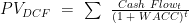
Notice that in this form it’s possible to use varying levels of the firm’s discount factor, WACC, for each year forecast, though absent information with respect to future interest, inflation and rates of return this is inadvisable. Also note that while an average annual rate of change of the subject cash flow variable is calculable, such rate is likely not used as the forecast resulting in the cash flow variable should be robust enough to consider future incomes and expenses.
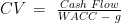
The firm’s continuing (terminal) value as of a future point in time is calculable as 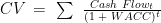
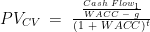
The present value of all of the asset’s future cash flows may then be calculated as 
This study explores the use of varying forms of cash flow in the explicit forecast period: Net Operating Profit Less Adjusted Taxes (NOPLAT), Net Income (NI), Free Cash Flow (FCF), Cash Flow from Equity (CFE) and the Tax Shield (TS). We also consider varying continuation period models, such Key Value Driver (KVD), Free Cash Flow (FCF) Adjusted Present Value (APV), Economic Profit (Eπ) and Forward Market Multiple (FMM). Each of the continuing value models employs variables for cash flow, discount factor, and growth. The discount factor used in this study is a market value based form of the asset’s Weighted Average Cost of Capital (WACC), though a book value based version of WACC is noted for each firm in the study.
A particular weakness of the continuation equation arises when g is greater than WACC resulting in an expressly negative valuation, which is often a spurious result and may not be credible.
1Richard Haskell, PhD (2017), Associate Professor of Finance, Bill & Vieve Gore School of Business, Westminster College, Salt Lake City, Utah, rhaskell@westminstercollege.edu, www.richardhaskell.net.
Time Signatures1
The time signatures used in the various models are important in that they specify for what period the variable value is to be employed and they often also form an exponent active in many of the models’ denominators. For the purposes of this study, we assume each calculated value is as of period zero (0) and that the explicit forecast period begins in period one (1) and continues through period t.
We will also assume that the continuation period begins at period t plus 1 (t + 1) and has no specified end. As we assign a value for these cash flows they are as of the end of the explicit period. In the continuing value equation, we refer to this as period zero (0), but it’s important to recall that this is the same as the last year of the explicit period and that the use of t = 1 in the continuation equations is the first year of the continuation period.
As an example, suppose we have a 5-year explicit period followed by an infinite continuation period. The equation and time signatures for this calculation are
![VAL\,\,=\,\,PV_{DCF}\,\,+\,\,PV_{CV}\,\,=\,\,\sum\big[\,\,\frac{Cash\,\,Flow_{1}}{(1\,\,+\,\,WACC)^{1}}\,\,+\,\,\frac{Cash\,\,Flow_{2}}{(1\,\,+\,\,WACC)^{2}}\,\,+\,\,\frac{Cash\,\,Flow_{3}}{(1\,\,+\,\,WACC)^{3}}\,\,+\,\,\frac{Cash\,\,Flow_{4}}{(1\,\,+\,\,WACC)^{4}}\,\,+\,\,\frac{Cash\,\,Flow_{5}}{(1\,\,+\,\,WACC)^{5}}\big]\,\,+\,\,\frac{\frac{Cash\,\,Flow_{1}}{WACC\,\,-\,\,g}}{(1\,\,+\,\,WACC)^{t}}](http://s0.wp.com/latex.php?latex=VAL%5C%2C%5C%2C%3D%5C%2C%5C%2CPV_%7BDCF%7D%5C%2C%5C%2C%2B%5C%2C%5C%2CPV_%7BCV%7D%5C%2C%5C%2C%3D%5C%2C%5C%2C%5Csum%5Cbig%5B%5C%2C%5C%2C%5Cfrac%7BCash%5C%2C%5C%2CFlow_%7B1%7D%7D%7B%281%5C%2C%5C%2C%2B%5C%2C%5C%2CWACC%29%5E%7B1%7D%7D%5C%2C%5C%2C%2B%5C%2C%5C%2C%5Cfrac%7BCash%5C%2C%5C%2CFlow_%7B2%7D%7D%7B%281%5C%2C%5C%2C%2B%5C%2C%5C%2CWACC%29%5E%7B2%7D%7D%5C%2C%5C%2C%2B%5C%2C%5C%2C%5Cfrac%7BCash%5C%2C%5C%2CFlow_%7B3%7D%7D%7B%281%5C%2C%5C%2C%2B%5C%2C%5C%2CWACC%29%5E%7B3%7D%7D%5C%2C%5C%2C%2B%5C%2C%5C%2C%5Cfrac%7BCash%5C%2C%5C%2CFlow_%7B4%7D%7D%7B%281%5C%2C%5C%2C%2B%5C%2C%5C%2CWACC%29%5E%7B4%7D%7D%5C%2C%5C%2C%2B%5C%2C%5C%2C%5Cfrac%7BCash%5C%2C%5C%2CFlow_%7B5%7D%7D%7B%281%5C%2C%5C%2C%2B%5C%2C%5C%2CWACC%29%5E%7B5%7D%7D%5Cbig%5D%5C%2C%5C%2C%2B%5C%2C%5C%2C%5Cfrac%7B%5Cfrac%7BCash%5C%2C%5C%2CFlow_%7B1%7D%7D%7BWACC%5C%2C%5C%2C-%5C%2C%5C%2Cg%7D%7D%7B%281%5C%2C%5C%2C%2B%5C%2C%5C%2CWACC%29%5E%7Bt%7D%7D&bg=ffffff&fg=000&s=0&c=20201002)
Note that t = 1 is used for the first term in the explicit forecast period as well as the first year of the continuation period suggesting that the last year of the explicit period is time = 0 for the continuation period.
1Richard Haskell, PhD (2017), Associate Professor of Finance, Bill & Vieve Gore School of Business, Westminster College, Salt Lake City, Utah, rhaskell@westminstercollege.edu, www.richardhaskell.net.